Clustering refers to the task of grouping similar instances or data points in a dataset. It is useful because it helps find underlying patterns in the dataset that may be useful for labeling data or gaining insights about the data.
We will be looking at two popular types of clustering.
k-Means Clustering
K-means clustering is a centroid-based clustering algorithm. Here, we assign a number of clusters, k, for the algorithm to find the clusters present in the dataset.
To find the clusters, we start by placing the centroids randomly. Then we start labeling the instances based on some cost function, such as Euclidean distance. Since the randomly assigned centroids may not be the actual centroids for each cluster, we start updating the centroids. This updating of centroids is done until they stop moving by more than a certain threshold or until a fixed number of steps is reached. As we are using the mean squared distance between the instances and their closest centroids, we can guarantee convergence because it cannot be negative. The steps below show how it actually occurs.
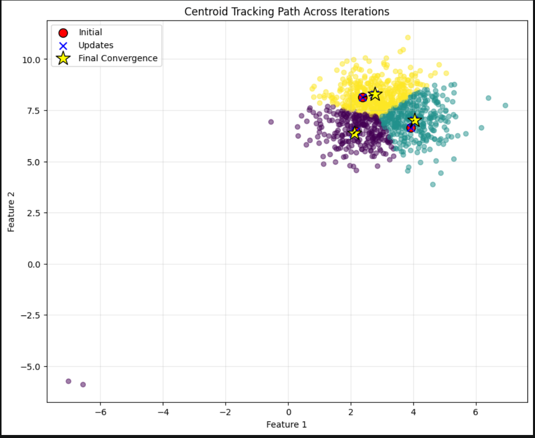
Although convergence is guaranteed in K-means, it may not converge to the right solution because, if we get unlucky during initialization, we may end up with a suboptimal solution.
For us to know which initialization performed the best, realistically there are two ways. Either we run a different clustering algorithm beforehand, which can then be used to somewhat estimate where the centroids may lie, or by running the clustering algorithm repeatedly, we can choose the initialization with the best performance metric.
Hmm… So how do we compare which solution is better? For this, we use a metric known as Inertia.
Inertia
$$ \text{Inertia}=\sum_i \left|x^{(i)}-c^{(i)}\right|^2 $$
Here, the (x^{(i)}) term represents a data point and (c^{(i)}) the nearest centroid to that data point. When summing up all the distances, a lower inertia results in better clustering. Hence, the initialization with the least inertia can be thought of as the better one.
Now, although we used inertia to find the better initialization for our problem, it is still too inefficient, right? We first have to select 10 random points, then calculate and repeat. It is too cumbersome and inefficient. So what we can use instead is K-means++ for initialization.
K-means++
The steps involved in K-means++ initialization are:
-
From a given dataset, take a single random point as the first centroid (c_1).
-
For each data point (x) in the dataset, compute its Euclidean distance to the nearest already selected centroid. Let this distance be (D(x)).
-
Choose one new data point at random as the next centroid using a weighted probability distribution, where the probability of choosing point (x) is proportional to its squared distance, (D(x)^2).
$$ \text{Probability}(x)= \frac{D(x)^2} {\sum_{x’}D(x’)^2} $$
-
Repeat until you have the required number of initial centroids.
Number of clusters (k) selection
For humans, looking at a 2D or 3D graph and distinguishing the clusters present is a simple enough task. However, in machine learning, it is difficult for a machine to intuitively know what the number of clusters should be.
Cluster selection remains a tricky task as well. It might be assumed that choosing the clustering algorithm with the least inertia value would give us the best selection of k, right?
Actually, inertia is bound to decrease as the value of k increases, which is why inertia is not the best metric to determine k.
Hmm… So what might be the way?
Let’s plot inertia against values of k to see how inertia decreases as k increases.
import matplotlib.pyplot as plt
from sklearn.cluster import KMeans
from sklearn.datasets import make_blobs
X,y=make_blobs([1000,2])
inertia_list=[]

for i in range(2,8):
	k=i
	kmeans=KMeans(n_clusters=k,random_state=42)
	y_pred=kmeans.fit_predict(X)
	inertia_list.append(kmeans.inertia_)

k_values=range(2,8)

plt.figure(figsize=(6, 4))
plt.plot(k_values, inertia_list, marker='o')
plt.xlabel("Number of Clusters (k)")
plt.ylabel("Inertia")
plt.title("Elbow Method")
plt.xticks(k_values)
plt.grid(True)
plt.show()
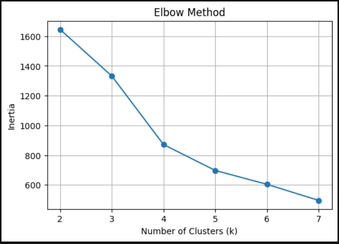
Here, we can see that we have a sharp change in the slope of the line at k = 4, which indicates that even though inertia is getting lower as the value of k increases, the rate at which it was decreasing has dramatically fallen.
We call this the elbow method, where we choose k by looking at the rate at which inertia decreases. Looking at the output, we can also see that 4 clusters is actually quite a valid choice.
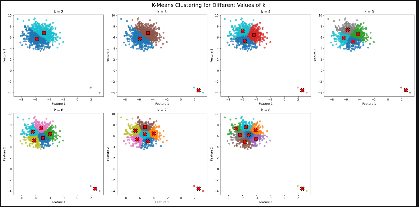
However, this method, although useful in many cases, might not always be precise. We might have cases where the slopes do not decrease at dramatically different rates, making it harder for us to determine the right value of k.
This is where the silhouette coefficient comes into play. The silhouette coefficient uses inter-cluster and intra-cluster distances to calculate the appropriate number of clusters, k.
Silhouette Score
The silhouette score for a single data point is calculated as:
$$ s(i)= \frac{b(i)-a(i)} {\max(a(i),,b(i))} $$
Where:
-
(s(i)): Silhouette score of data point (i).
-
(a(i)): The average distance between data point (i) and all other points in the same cluster (intra-cluster distance).
-
(b(i)): The smallest average distance between data point (i) and all points in any other cluster (nearest-cluster distance).
-
(s(i)\approx1): The point is well clustered and far from neighboring clusters.
-
(s(i)\approx0): The point lies close to the boundary between two clusters.
-
(s(i)<0): The point may have been assigned to the wrong cluster.
These scores for every data point in a cluster are then averaged using the formula
$$ S=\frac{1}{N}\sum_{i=1}^{N}s(i) $$
for each cluster.
Meaning, we get to know the silhouette score for each value of k in a range of k values. The one with the highest silhouette score is then chosen.
For the above example, if we were to calculate the silhouette scores, we would get:
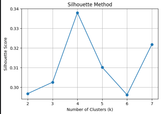
which further verifies that, indeed, k = 4 results in better clustering.